Ethnobotanical Leaflets 13: 234-48. 2009.
Study on the Distribution of Flora and Fauna in the SIPCOT Industrial Park of Gangaikondan, Tirunelvelli District, Tamil Nadu, India
Jegan G and Muthuchelian K*
Centre for Biodiversity and Forest studies, Department of Bioenergy
School of Energy, Environmental and Natural Resources, Madurai Kamaraj University
Madurai – 625 021, Tamil Nadu, India
*Corresponding Author: [email protected]
Issued 30 January 2009
Abstract
The phytosociological study on flora and fauna diversity in Gangaikondan revealed that the diversity of the flora was more than the faunal diversity. Totally 59 floral species and 35 faunal species were listed out in the study site. For plants the species- area curves attained the stable position in 2nd and 3rd quadrats where for fauna it reached the observed species richness in 4th and 5th quadrats.
Keywords: Gangaikondan, fauna, flora, SIPCOT.
Introduction
Biological surveys, focusing on species diversity, are necessary on both national and global scales. National biological inventories provide a finer-grained view of biological diversity and can be used to establish national conservation programs and policies, whereas a global survey will provide much needed information on the extent, distribution, status, and fate of biodiversity worldwide. These efforts can serve not only to tell us the status of biodiversity, but to identify valuable biological resources, some of which are unknown, while others are locally known but have potential for much wider use. Many plants of current or potential commercial value were discovered in the course of routine plant surveys. Inventories and surveys also provide baseline data against which to monitor changes in biological diversity and to trace the environmental impacts of development projects.
In recent years a great deal of interest has surfaced in the quantification and valuation of biological diversity. The interest is largely motivated by findings from natural scientists that biodiversity is imperiled by human activities (Wilson 1992), especially the destruction of natural habitats (Primack 2000). Biodiversity has, however, proved both difficult to define in practice and difficult to relate to human welfare. Definition and valuation are closely related, of course. We cannot speak meaningfully of valuation without having some notion of what it is that is being valued. On the other hand, a definition that cannot be related to human values may propose “distinctions without differences.”
Objective of our study was to screen the list of flora and fauna of the SIPCOT Industrial Park.
Materials and Methods
Study Site
The study site was SIPCOT industrial park of Gangaikondan, Tirunelvelli District, Tamil Nadu, India.
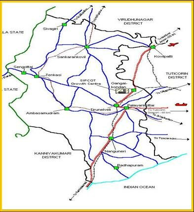
Map 1: Map showing the study site.
Sampling
In the SIPCOT Industrial Park the phytosociological study was carried out using 12 randomly placed quadrats (10m´10m) for trees (individual with DBH more than 30 cm) within them 5m´5m for shrubs and climbers and 1m´1m for herbaceous community.
Analysis
The diversity indices were analyzed using PAST and Biodiversity Pro beta Version 2. The species- area were raised with the help of EstimateS.
Chao 1: An abundance-based estimator of species richness
Jackknife 1: First-order jackknife estimator of species richness (incidence-based)
ACE: Abundance-based Coverage Estimator of species richness
Bootstrap: Bootstrap estimator of species richness (incidence-based)
ICE: Incidence-based Coverage Estimator of species richness
Results and Discussion
Floral Diversity
In the SIPCOT Industrial Park totally 59 plant species were found. Totally 972 individuals were representing 59 species. Borassus flabellifer L. was the dominant species among 59 species. Cyperus rotundus L. was having lower number of individuals (4). Cuscuta sp. a parasitic species was occurred in the proposed site which was a nuisance one to the common species like Azadiracta indica.
Diversity Indices
The diversity indices calculated for the SIPCOT Industrial Park showed the higher diversity of plant species. The dominance index of the proposed study site was 0.04. The Menhinick diversity index was also go hand with the Shannon index (Table 2).
Species – area curve
The assumption is that the species-area curves should reach the classic asymptotic form at assumption is that the species-area curves should reach the classic asymptotic form at a very early stage and forms a plateau (Chazdon et al., 1999).
In the SIPCOT Industrial Park, the species – area curves got stabled within 2nd and 3rd quadrats (Fig 1).
Principal Component Analysis
Principal component analysis was carried out by considering the distribution of species in the samples. Most of the species of the project site were following the similar pattern of distribution (Fig 2).
Correlations
Kulczynski Comparison was used for assessing species turnover between samples. Spearman's rank correlation coefficient was used to test for relationship between samples. The Mann-Whitney U test was a non-parametric ranking test for whether two independent random samples are drawn from populations having the same distributions. The variance-covariance matrix showed the variance of each sample in the leading (main) diagonal of the matrix and the sample by sample covariance in the other cells.
Faunal Diversity
In the SIPCOT Industrial Park totally 35 faunal species were found. Totally 504 individuals were representing 35 species. Bufo melanostictus was the dominant species among 35 species. Danaus chrysippus and Acantholepis were having lower number of individuals (7).
Diversity Indices
The diversity indices calculated for the SIPCOT Industrial Park showed the higher diversity of animal species. The dominance index of the proposed study site was 0.07. The Menhinick diversity index was also go hand with the Shannon index (Table 7).
Species – area curve
The assumption is that the species-area curves should reach the classic asymptotic form at assumption is that the species-area curves should reach the classic asymptotic form at a very early stage and forms a plateau (Chazdon et al., 1999).
In the SIPCOT Industrial Park, the species – area curves got stabled within 4th and 5th quadrats (Fig 3).
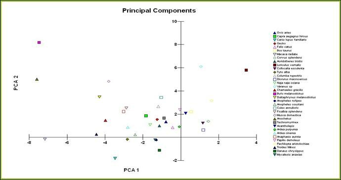
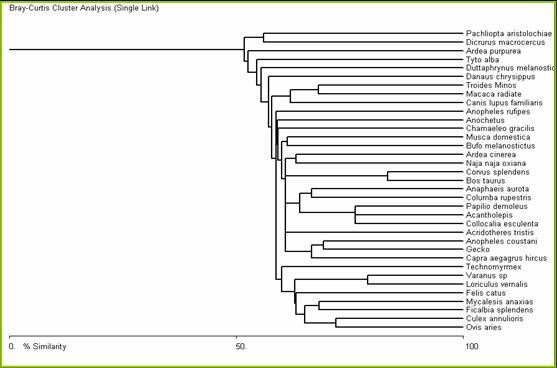
Principal Component Analysis and Cluster Analysis
Principal component analysis was carried out by considering the distribution of species in the samples. Most of the species of the project site were differed in their pattern of distribution (Fig 4). Most of the species showed above 50% of similarity in their distribution (Fig 5).
Table 1: List of flora in the in the SIPCOT Industrial Park and its surroundings.
S.No. |
Botanical Name |
Common Name |
|
Azadiracta indica A. Juss. |
Vembu |
|
Boerhhavia diffusa L. |
|
|
Calotropis gigantea (L.) R.Br. |
Eruku |
|
Borassus flabellifer L. |
Panai |
|
Cassia siamea Lam. |
|
|
Cissus quadrangularis L. |
Nanmuga pirandai |
|
Clerodendrum inerme (L.) Gaertn |
|
|
Cleome gynandra L. |
|
|
Cleome viscosa L. |
Naikaduku |
|
Cocos nucifera L. |
Thenai |
|
Commelina benghalensis L. |
Thankaipoo |
|
Cynodon dactylon (L.) Pers. |
Arukanpull |
|
Cyperus rotundus L. |
|
|
Cassia fistula L. |
Sarakonai |
|
Ficus benghalensis L. |
Alamaram |
|
Ficus religiosa L. |
Arasamaram |
|
Indigofera uniflora Buch. |
|
|
Moringa pterygosperma Goertn. |
Murungai |
|
Jasminum angustifolium (L.) Willd. |
Malligai |
|
Mangifera indica L. |
Mango |
|
Ficus racemosa |
|
|
Delonix regia (Boj. ex Hook.) Raf. |
Myilkonrai |
|
Carica papaya L. |
Pappali |
|
Ocimum sanctum |
Tulsi |
|
Pergularia daemia L |
Veliparuthi |
|
Parthenium hysterophorus L. |
Parthenium |
|
Abutilon indicum (Linn.) Sweet. |
Thuthi |
|
Tribulus terrestris Linn |
Nerunji |
|
Prosopis julifera |
Karuvelam |
S.No. |
Botanical Name |
Common Name |
|
Polyalthia longifolia (Sonner) Thw. |
Nedulingam |
|
Tamarindus indica L. |
Puli |
|
Thespesia populanea (L.) Soland. |
Poovarasu |
|
Aloe vera (L.) Burm.f. |
Sodrukathalai |
|
Ricinus communis L. |
Athalai |
|
Croton sparsiflorus Morong |
|
|
Opuntia |
Kalli |
|
Ziziphus |
|
|
Aerva lanata (L.) Juss. ex. Sch. |
Kanupula sedi |
|
Cassia auriculata L. |
Avarai |
|
Morinda tinctoria Roxb |
Manchanathi |
|
Cuscuta L. |
|
|
Tectona grandis L. f. |
Thekku |
|
Hibiscus rosa-sinensis L. |
Chembaruthi |
|
Acacia planiformis Wight & Arn |
Odaimaram |
|
Samanea samen (Jacq.) Marrill. |
Thungumungi maram |
|
Millingtonia hortensis L. |
Pannerpoomaram |
|
Tridax procumbens L |
|
|
Leucaena leucocephala (Lamk) Wit. |
Subapull |
|
Agave americana L. |
|
|
Albizzia lebbeck Benth. |
Vagai |
|
Terminalia catappa L. |
Vatham |
|
Typha latifolia |
|
|
Achyranthes aspera |
Nayuruvi |
|
Jatropha gossifolia |
|
|
Musa paradisiaca L. |
Vallai |
|
Bougainvillea spectabilis |
Kakithapoo |
|
Eucalyptus |
|
|
Marsilea |
|
|
Arundina |
|
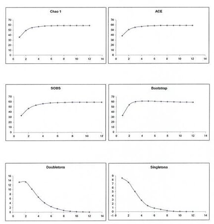
Fig 1: Observed and Estimated area – curves of the SIPCOT Industrial Park.
Table 2: Consolidated details on the floral diversity of the SIPCOT Industrial Park.
Number of Species |
59 |
Number of Individuals |
972 |
Dominance |
0.041 |
Shannon Diversity |
3.33 |
Simpson |
0.95 |
Evenness |
0.86 |
Menhinick |
3.64 |
Margalef |
7.23 |
Equitability index |
0.95 |
Fisher alpha diversity |
20.77 |
Berger-Parker |
0.08 |
Fig 2: Principal Component Analysis of floral species distribution in the SIPCOT Industrial Park. Refer table 1 for the species list.
Table 3: Kulczynski Comparison
|
Sample 1 |
Sample 2 |
Sample 3 |
Sample 4 |
Sample 5 |
Sample 6 |
Sample 7 |
Sample 8 |
Sample 9 |
Sample 10 |
Sample 11 |
Sample 12 |
Sample 1 |
* |
* |
* |
* |
* |
* |
* |
* |
* |
* |
* |
* |
Sample 2 |
35 |
* |
* |
* |
* |
* |
* |
* |
* |
* |
* |
* |
Sample 3 |
64.17 |
40.66 |
* |
* |
* |
* |
* |
* |
* |
* |
* |
* |
Sample 4 |
56.47 |
59.71 |
48.61 |
* |
* |
* |
* |
* |
* |
* |
* |
* |
Sample 5 |
60 |
50.91 |
61.11 |
43.92 |
* |
* |
* |
* |
* |
* |
* |
* |
Sample 6 |
58.13 |
49.24 |
64.93 |
66.73 |
38.75 |
* |
* |
* |
* |
* |
* |
* |
Sample 7 |
63.38 |
57.33 |
71.25 |
53.62 |
66.4 |
46.62 |
* |
* |
* |
* |
* |
* |
Sample 8 |
63.33 |
54.09 |
61.11 |
53.33 |
60 |
51.67 |
57.34 |
* |
* |
* |
* |
* |
Sample 9 |
65.61 |
59.45 |
64.91 |
52.94 |
65.61 |
54.69 |
64.01 |
53.68 |
* |
* |
* |
* |
Sample 10 |
67.81 |
58.48 |
61.98 |
63.69 |
64.58 |
53.13 |
67.02 |
54.9 |
63.32 |
* |
* |
* |
Sample 11 |
65.59 |
56.3 |
51.03 |
55.5 |
45.91 |
60.33 |
59.29 |
62.31 |
61.5 |
44.46 |
* |
* |
Sample 12 |
46.67 |
57.27 |
61.11 |
40.78 |
63.33 |
54.9 |
69.41 |
53.33 |
59.65 |
58.13 |
42.63 |
* |
Table 4: Rank Correlation
|
Sample 1 |
Sample 2 |
Sample 3 |
Sample 4 |
Sample 5 |
Sample 6 |
Sample 7 |
Sample 8 |
Sample 9 |
Sample 10 |
Sample 11 |
Sample 12 |
Sample 1 |
1 |
* |
* |
* |
* |
* |
* |
* |
* |
* |
* |
* |
Sample 2 |
-0.1408 |
1 |
* |
* |
* |
* |
* |
* |
* |
* |
* |
* |
Sample 3 |
0.3381 |
-0.2732 |
1 |
* |
* |
* |
* |
* |
* |
* |
* |
* |
Sample 4 |
0.2249 |
0.1709 |
0.0907 |
1 |
* |
* |
* |
* |
* |
* |
* |
* |
Sample 5 |
0.2907 |
0.1201 |
0.2398 |
-0.0546 |
1 |
* |
* |
* |
* |
* |
* |
* |
Sample 6 |
0.2179 |
0.1652 |
0.3137 |
0.3891 |
-0.0705 |
1 |
* |
* |
* |
* |
* |
* |
Sample 7 |
0.3009 |
-0.0091 |
0.2353 |
0.0591 |
0.2849 |
-0.1951 |
1 |
* |
* |
* |
* |
* |
Sample 8 |
0.4626 |
0.1044 |
0.2376 |
0.1292 |
0.328 |
0.1809 |
0.1102 |
1 |
* |
* |
* |
* |
Sample 9 |
0.2162 |
0.1196 |
0.2846 |
-0.0256 |
0.2999 |
0.0856 |
0.1271 |
0.1475 |
1 |
* |
* |
* |
Sample 10 |
0.5101 |
0.0689 |
0.3127 |
0.2721 |
0.2896 |
0.1298 |
0.3712 |
0.2214 |
0.1771 |
1 |
* |
* |
Sample 11 |
0.323 |
0.1352 |
0.1026 |
0.2227 |
0.0639 |
0.2384 |
0.1558 |
0.2088 |
0.2485 |
0.127 |
1 |
* |
Sample 12 |
-0.0108 |
0.2924 |
0.1059 |
-0.1334 |
0.4251 |
0.133 |
0.3012 |
0.2416 |
0.2356 |
0.2023 |
0.0156 |
1 |
Table 5: Mann- Whitney
|
Sample 1 |
Sample 2 |
Sample 3 |
Sample 4 |
Sample 5 |
Sample 6 |
Sample 7 |
Sample 8 |
Sample 9 |
Sample 10 |
Sample 11 |
Sample 12 |
Sample 1 |
* |
* |
* |
* |
* |
* |
* |
* |
* |
* |
* |
* |
Sample 2 |
422 |
* |
* |
* |
* |
* |
* |
* |
* |
* |
* |
* |
Sample 3 |
534 |
502 |
* |
* |
* |
* |
* |
* |
* |
* |
* |
* |
Sample 4 |
488 |
494 |
598 |
* |
* |
* |
* |
* |
* |
* |
* |
* |
Sample 5 |
367 |
310 |
410 |
384 |
* |
* |
* |
* |
* |
* |
* |
* |
Sample 6 |
442 |
398 |
510 |
474 |
429 |
* |
* |
* |
* |
* |
* |
* |
Sample 7 |
516 |
464 |
592 |
550 |
490 |
590 |
* |
* |
* |
* |
* |
* |
Sample 8 |
412 |
366 |
468 |
438 |
408 |
474 |
547 |
* |
* |
* |
* |
* |
Sample 9 |
518 |
461 |
599 |
558 |
511 |
608 |
697 |
561 |
* |
* |
* |
* |
Sample 10 |
428 |
380 |
496 |
458 |
438 |
502 |
574 |
476 |
600 |
* |
* |
* |
Sample 11 |
452 |
403 |
535 |
498 |
368 |
450 |
526 |
410 |
531 |
446 |
* |
* |
Sample 12 |
348 |
284 |
376 |
356 |
420 |
401 |
457 |
380 |
476 |
410 |
333 |
* |
Table 6: Variance – Covariance
|
Sample 1 |
Sample 2 |
Sample 3 |
Sample 4 |
Sample 5 |
Sample 6 |
Sample 7 |
Sample 8 |
Sample 9 |
Sample 10 |
Sample 11 |
Sample 12 |
Sample 1 |
3.6014 |
* |
* |
* |
* |
* |
* |
* |
* |
* |
* |
* |
Sample 2 |
-0.3141 |
2.4535 |
* |
* |
* |
* |
* |
* |
* |
* |
* |
* |
Sample 3 |
0.9696 |
-0.5269 |
2.1297 |
* |
* |
* |
* |
* |
* |
* |
* |
* |
Sample 4 |
0.3939 |
0.3326 |
0.2122 |
2.1321 |
* |
* |
* |
* |
* |
* |
* |
* |
Sample 5 |
0.6715 |
0.72 |
0.3983 |
-0.2721 |
3.1794 |
* |
* |
* |
* |
* |
* |
* |
Sample 6 |
0.4191 |
1.6108 |
0.9205 |
0.7358 |
0.8545 |
4.1835 |
* |
* |
* |
* |
* |
* |
Sample 7 |
1.0009 |
-0.358 |
0.3603 |
0.1514 |
0.6826 |
-0.8717 |
2.7656 |
* |
* |
* |
* |
* |
Sample 8 |
1.2271 |
0.4906 |
0.4424 |
-0.0357 |
0.9077 |
0.8816 |
0.3165 |
2.3308 |
* |
* |
* |
* |
Sample 9 |
0.1739 |
0.8746 |
0.5488 |
-0.3109 |
1.0918 |
1.0529 |
0.322 |
0.5792 |
2.893 |
* |
* |
* |
Sample 10 |
1.5798 |
-0.2484 |
1.0473 |
0.6888 |
0.2756 |
0.1397 |
0.7934 |
0.3515 |
0.2706 |
3.1473 |
* |
* |
Sample 11 |
0.3349 |
-0.1613 |
0.0544 |
0.3936 |
-0.0929 |
0.0921 |
0.2826 |
0.0856 |
0.3273 |
0.353 |
1.5675 |
* |
Sample 12 |
-0.6099 |
0.7688 |
-0.0561 |
-0.5181 |
1.1376 |
0.5362 |
0.6037 |
0.4205 |
1.0465 |
0.13 |
-0.1125 |
2.8369 |
List of Fauna in the in the SIPCOT Industrial Park and its surroundings
Table 7: Consolidated details on the faunal diversity in the SIPCOT Industrial Park
Number of species |
35 |
Number of Individuals |
504 |
Dominance |
0.07 |
Shannon index |
2.70 |
Simpson index |
0.92 |
Evenness |
0.86 |
Menhinick |
2.73 |
Margalef |
4.46 |
Equitability index |
0.94 |
Fisher alpha diversity |
11.74 |
Berger-Parker |
0.131251 |
Fig 3: Observed and estimated species – area curves of fauna in the SIPCOT Industrial Park
Fig 4: Principal Component Analysis of faunal species distribution in the SIPCOT
Industrial Park.
Fig 4: Fig 5: Cluster diagram produced by the distribution of faunal species in the SIPCOT Industrial Park. n the SIPCOT Industrial Park.
![]() |
Table 8: Kulczynski Comparison
|
Sample 1 |
Sample 2 |
Sample 3 |
Sample 4 |
Sample 5 |
Sample 6 |
Sample 7 |
Sample 8 |
Sample 9 |
Sample 10 |
Sample 11 |
Sample 12 |
Sample 1 |
* |
* |
* |
* |
* |
* |
* |
* |
* |
* |
* |
* |
Sample 2 |
26.39 |
* |
* |
* |
* |
* |
* |
* |
* |
* |
* |
* |
Sample 3 |
61.58 |
32.46 |
* |
* |
* |
* |
* |
* |
* |
* |
* |
* |
Sample 4 |
50 |
52.78 |
46.18 |
* |
* |
* |
* |
* |
* |
* |
* |
* |
Sample 5 |
43.53 |
62.91 |
44.58 |
54.41 |
* |
* |
* |
* |
* |
* |
* |
* |
Sample 6 |
65.43 |
59.42 |
76.89 |
56.09 |
46.04 |
* |
* |
* |
* |
* |
* |
* |
Sample 7 |
42.5 |
44.44 |
55.83 |
42.5 |
39.08 |
40.22 |
* |
* |
* |
* |
* |
* |
Sample 8 |
54.41 |
51.47 |
55.73 |
43.53 |
64.71 |
51.15 |
52.1 |
* |
* |
* |
* |
* |
Sample 9 |
55 |
63.33 |
46.18 |
55 |
65.29 |
46.74 |
42.5 |
54.41 |
* |
* |
* |
* |
Sample 10 |
65.29 |
45.75 |
61.3 |
48.97 |
52.94 |
61.38 |
39.08 |
52.94 |
54.41 |
* |
* |
* |
Sample 11 |
54.64 |
38.1 |
37.22 |
54.64 |
52.1 |
45.96 |
57.14 |
58.61 |
36.43 |
26.05 |
* |
* |
Sample 12 |
44.42 |
52.99 |
45.34 |
31.73 |
47.51 |
60.2 |
59.34 |
54.3 |
44.42 |
33.94 |
37.09 |
* |
Table 9: Rank Correlation
|
Sample 1 |
Sample 2 |
Sample 3 |
Sample 4 |
Sample 5 |
Sample 6 |
Sample 7 |
Sample 8 |
Sample 9 |
Sample 10 |
Sample 11 |
Sample 12 |
Sample 1 |
1 |
* |
* |
* |
* |
* |
* |
* |
* |
* |
* |
* |
Sample 2 |
-0.2965 |
1 |
* |
* |
* |
* |
* |
* |
* |
* |
* |
* |
Sample 3 |
0.2432 |
-0.2781 |
1 |
* |
* |
* |
* |
* |
* |
* |
* |
* |
Sample 4 |
-0.1931 |
0.0992 |
-0.1564 |
1 |
* |
* |
* |
* |
* |
* |
* |
* |
Sample 5 |
-0.1736 |
0.4461 |
-0.0585 |
0.1696 |
1 |
* |
* |
* |
* |
* |
* |
* |
Sample 6 |
0.1095 |
0.2658 |
0.3797 |
0.119 |
0.1305 |
1 |
* |
* |
* |
* |
* |
* |
Sample 7 |
0.0626 |
0.1178 |
0.1882 |
0.1729 |
0.1499 |
-0.2383 |
1 |
* |
* |
* |
* |
* |
Sample 8 |
0.1022 |
0.1034 |
0.2963 |
-0.0303 |
0.4698 |
0.0032 |
0.2838 |
1 |
* |
* |
* |
* |
Sample 9 |
-0.1734 |
0.3221 |
0.0091 |
-0.0851 |
0.4123 |
-0.0065 |
0.0632 |
0.1949 |
1 |
* |
* |
* |
Sample 10 |
0.4336 |
-0.0174 |
0.3579 |
-0.0537 |
0.1733 |
0.2 |
0.0519 |
0.1997 |
0.0286 |
1 |
* |
* |
Sample 11 |
0.1177 |
0.1141 |
-0.0479 |
0.3098 |
0.3665 |
-0.0052 |
0.3706 |
0.3638 |
-0.0653 |
-0.0152 |
1 |
* |
Sample 12 |
0.0685 |
0.3791 |
0.2636 |
-0.0141 |
0.3849 |
0.2704 |
0.5029 |
0.4091 |
0.2279 |
0.0721 |
0.182 |
1 |
Table 10: Mann- Whitney
|
Sample 1 |
Sample 2 |
Sample 3 |
Sample 4 |
Sample 5 |
Sample 6 |
Sample 7 |
Sample 8 |
Sample 9 |
Sample 10 |
Sample 11 |
Sample 12 |
Sample 1 |
* |
* |
* |
* |
* |
* |
* |
* |
* |
* |
* |
* |
Sample 2 |
179 |
* |
* |
* |
* |
* |
* |
* |
* |
* |
* |
* |
Sample 3 |
169 |
152 |
* |
* |
* |
* |
* |
* |
* |
* |
* |
* |
Sample 4 |
196 |
176 |
164 |
* |
* |
* |
* |
* |
* |
* |
* |
* |
Sample 5 |
166 |
150 |
140 |
170 |
* |
* |
* |
* |
* |
* |
* |
* |
Sample 6 |
179 |
162 |
141 |
182 |
153 |
* |
* |
* |
* |
* |
* |
* |
Sample 7 |
129 |
118 |
107 |
135 |
112 |
131 |
* |
* |
* |
* |
* |
* |
Sample 8 |
134 |
122 |
102 |
136 |
113 |
192 |
94 |
* |
* |
* |
* |
* |
Sample 9 |
166 |
152 |
134 |
175 |
143 |
208 |
125 |
148 |
* |
* |
* |
* |
Sample 10 |
166 |
151 |
140 |
166 |
144 |
146 |
110 |
102 |
138 |
* |
* |
* |
Sample 11 |
128 |
118 |
104 |
135 |
110 |
130 |
94 |
90 |
132 |
103 |
* |
* |
Sample 12 |
90 |
84 |
66 |
96 |
76 |
145 |
65 |
110 |
106 |
68 |
67 |
* |
Table 11: Variance – Covariance
|
Sample 1 |
Sample 2 |
Sample 3 |
Sample 4 |
Sample 5 |
Sample 6 |
Sample 7 |
Sample 8 |
Sample 9 |
Sample 10 |
Sample 11 |
Sample 12 |
Sample 1 |
3.0555 |
* |
* |
* |
* |
* |
* |
* |
* |
* |
* |
* |
Sample 2 |
-0.7176 |
2.7529 |
* |
* |
* |
* |
* |
* |
* |
* |
* |
* |
Sample 3 |
0.3723 |
-0.8294 |
1.6168 |
* |
* |
* |
* |
* |
* |
* |
* |
* |
Sample 4 |
-0.9933 |
0.4353 |
-0.5975 |
2.5748 |
* |
* |
* |
* |
* |
* |
* |
* |
Sample 5 |
-0.9521 |
0.8294 |
-0.1798 |
0.3748 |
2.4571 |
* |
* |
* |
* |
* |
* |
* |
Sample 6 |
-0.195 |
1.1412 |
0.6504 |
0.6252 |
1.0429 |
3.7513 |
* |
* |
* |
* |
* |
* |
Sample 7 |
-0.058 |
0.0176 |
-0.2034 |
0.0571 |
-0.0193 |
-0.9807 |
1.963 |
* |
* |
* |
* |
* |
Sample 8 |
-0.3361 |
-0.1176 |
0.521 |
-0.3866 |
1.0546 |
-0.084 |
0.4664 |
2.5042 |
* |
* |
* |
* |
Sample 9 |
-0.9748 |
0.7647 |
-0.0714 |
-0.7563 |
0.8319 |
0.3151 |
0.1555 |
0.4328 |
2.6639 |
* |
* |
* |
Sample 10 |
0.637 |
-0.3882 |
0.7345 |
-0.5387 |
-0.2975 |
0.0622 |
-0.321 |
0.3445 |
-0.4832 |
1.8521 |
* |
* |
Sample 11 |
-0.3613 |
-0.0882 |
-0.4076 |
0.3697 |
0.3992 |
-0.2521 |
0.2521 |
0.3655 |
-0.5252 |
-0.3193 |
1.4202 |
* |
Sample 12 |
-0.2353 |
0.6765 |
0.1471 |
-0.3824 |
0.8824 |
0.3529 |
0.8824 |
0.7647 |
0.6176 |
-0.2353 |
-0.1471 |
2.1176 |
Acknowledgements
We thank UGC for their financial support of this project. We also thank Mr. Nagaraj for his help during the field study. Our sincere thank to Tamil Nadu Forest Department for their permission.
References
Colwell, R. K. (1997). EstimateS: Statistical estimation of species richness andshared
species from samples. Version 5. User’s Guide and application published at: http://viceroy.eeb.uconn.edu/estimates
McAleece, N. (1997). BioDiversity Pro. Beta version 2. The Natural Museum of Natural
History and The Scottish Association for Marine Sciences, United Kingdom (http://[email protected] or http://www.nhm.ac.uk/zoology/bdpro).